Building a Python Crypto Scalper with Live Level 2 Market Data

There is a huge difference between building a trading bot that places trades and building one that has any realistic chance of making money.

Recently I started a new Python project with a fairly straightforward goal:

Build a fast crypto scalper that can watch live market microstructure, identify short-term opportunities and automatically enter and exit small trades.

The original idea was deliberately simple. Rather than trying to predict whether Bitcoin would be higher tomorrow, I wanted to look at extremely short-term movements — seconds rather than hours — and see whether information from the live order book and trade tape could provide enough of an edge for frequent small trades.

The result has turned into a much more interesting engineering project than I initially expected.

The basic idea

The application currently connects to OKX and consumes live market data for instruments such as:

BTC-USDT-SWAP
ETH-USDT-SWAP
SOL-USDT-SWAP

The system uses the exchange’s live WebSocket feeds rather than repeatedly polling REST endpoints.

That gives us access to data such as:

best bid and ask
Level 2 order-book depth
public trades
aggressive buy and sell volume
spread
short-term price movement
market depth imbalance
microprice pressure
realised volatility
trading activity

The application then converts this stream into a set of continuously updated features that the trading engine can evaluate.

The important part is that this is not a candle-based strategy.

A one-minute candlestick throws away an enormous amount of information. For a strategy that may only hold a position for 10 or 20 seconds, the events happening inside that candle are potentially much more important than the candle itself.

Building the trading workstation

The project is a Python desktop application with a PySide6 interface.

The current workstation includes separate views for:

Positions
Orders
OKX connection status
Level 2 market microstructure
Research data
Future outcome analysis
Edge research
Fast Scalping

The application starts its market-data connections automatically and records feature snapshots locally while it runs.

A simplified version of the architecture looks like this:

OKX WebSockets
      |
      +---- Ticker
      |
      +---- Level 2 Order Book
      |
      +---- Public Trade Tape
               |
               v
        Market Data Engine
               |
               v
          Feature Engine
               |
               v
        Fast Scalp Strategy
               |
        +------+------+
        |             |
        v             v
   Risk Engine    Paper Execution
                      |
                      v
                Trade Evidence
                      |
                      v
                 SQLite / CSV

The separation between the market-data layer, strategy and execution simulator has been important.

It means we can keep changing the strategy without rewriting the WebSocket infrastructure every time.

Looking inside the order book

One of the more interesting parts of the project is the microstructure view.

Rather than simply displaying the current Bitcoin price, the application reconstructs the Level 2 book and calculates metrics such as order-book imbalance.

For example, if the top levels of the book contain significantly more bid liquidity than ask liquidity, the imbalance becomes positive.

Conceptually:

Bid depth = 1,250 BTC
Ask depth =   750 BTC

Imbalance =
(Bid - Ask) / (Bid + Ask)

= 0.25

That does not mean the price is guaranteed to rise.

Large orders can disappear, liquidity can be spoofed, and aggressive trades can overwhelm the resting book.

But when book imbalance is combined with actual trades, it becomes considerably more useful.

Trade delta and aggressive flow

The application also tracks public trades and attempts to measure whether buyers or sellers are currently being more aggressive.

For example:

Aggressive buys:  180
Aggressive sells: 100

That creates positive trade delta.

We calculate this across several windows, including roughly:

1 second
5 seconds
30 seconds

This gives the strategy both an immediate signal and some context.

A sudden burst of aggressive buyers means something different if the previous 30 seconds were strongly bearish.

The scoring engine

The first automated version uses a directional score ranging approximately from:

-100 = strongly bearish

   0 = neutral

+100 = strongly bullish

The score combines several live features including:

1-second trade delta
5-second trade delta
30-second trade delta
Level 2 imbalance
short-term momentum
microprice pressure
volume acceleration

A sufficiently strong positive score can generate a Long signal, while a strong negative score can generate a Short signal.

The application also allows the trader to explicitly choose:

Long
Short
Both

For much of the recent testing I have concentrated on Long-only trading.

That has turned out to be useful because Long and Short signals do not necessarily behave symmetrically.

Maker-first execution

One of the biggest lessons from this project has been that fees can destroy a scalping strategy surprisingly quickly.

Initially the idea was simply:

Signal
  |
  v
Enter
  |
  v
Take a small profit
  |
  v
Repeat

The problem is that every entry and exit costs money.

On the OKX demo account used during testing, the API reported approximately:

Maker: 2 bps per side
Taker: 5 bps per side

One basis point is 0.01%.

A maker entry followed by a maker exit therefore has a theoretical fee floor of around:

4 bps round trip

A maker entry followed by a taker exit costs considerably more.

This immediately creates a major problem for a strategy trying to capture 1 or 2 basis points.

Even if the direction is correct, the trade can still lose money.

Why maker orders matter

The strategy therefore uses a maker-first entry model.

For a Long:

Current bid:  75,900.00
Current ask:  75,900.10

Place BUY at:
75,900.00

The simulator does not simply assume the order fills.

The market must actually come back and trade through or touch the resting order during the configured entry lifetime.

If it does not fill, the order expires.

This has another interesting consequence: maker orders introduce adverse-selection risk.

A resting buy order is often filled precisely because sellers are moving into it.

That means a maker fill is not necessarily the free advantage it initially appears to be.

This is something the project is now explicitly investigating.

Paper trading before real execution

Although the application uses live OKX market data and authenticates against a demo account, automated execution is currently deliberately restricted to paper trading.

That gives us:

Live market data
+
Live order book
+
Live trade tape
+
Simulated orders

without risking real capital while the strategy is still being developed.

Every completed simulated trade records information including:

entry time
exit time
side
entry score
exit score
entry price
exit price
hold duration
gross P&L
fees
net P&L
exit reason

More recently, we started recording much more detailed path information as well.

MFE and MAE

Two particularly useful metrics are:

MFE — Maximum Favourable Excursion

How far the trade moved in our favour while it was open.

MAE — Maximum Adverse Excursion

How far it moved against us.

Suppose we enter Bitcoin Long and the trade behaves like this:

Entry       75,900

Low         75,888
High        75,938
Exit        75,920

The exit price alone doesn’t tell us the full story.

The trade may have had enough potential profit to justify a different exit strategy.

Recording MFE and MAE allows us to ask questions like:

Are our targets too ambitious?
Are stops too tight?
Are we exiting profitable trades too early?
Do losing trades immediately move against us?
How much movement normally exists after a strong signal?

We also record approximate prices after:

1 second
3 seconds
5 seconds
10 seconds
20 seconds

That is proving extremely useful.

A surprising result

One of the recent Long-only tests produced a result that initially looked promising.

Of 12 completed trades:

9 / 12 were positive before fees

The average trade captured positive price movement.

At around five seconds after entry, most positions were also still moving in the expected direction.

That sounds great.

Except the magnitude was tiny.

The average maximum favourable movement was only around a few basis points.

The best trade moved a little over 6 bps in our favour.

The problem was the fee floor.

A strategy can therefore be right surprisingly often and still lose money.

That is probably the most useful lesson from the project so far.

Accuracy alone is not enough.

The actual equation is closer to:

Trading Edge
-
Fees
-
Spread
-
Slippage
-
Adverse Selection
=
Real Edge

If the result is negative, a 90% directional hit rate is irrelevant.

Dynamic exits

Another early version of the strategy waited for either:

take profit
stop loss
maximum hold time

That turned out to be too simplistic for very short-term trading.

Imagine a Long position was entered with a strong score of:

+70

Five seconds later the score collapses to:

+5

and then becomes:

-30

The reason for entering the trade has disappeared.

Waiting another 15 seconds for a fixed stop or target makes very little sense.

The current strategy therefore supports dynamic exits.

A position can now exit because:

the hard profit target is reached
the stop is reached
the maximum holding period expires
the microstructure signal fades
a strong opposite signal persists
an existing profit needs protecting

Reversal logic also includes persistence.

The engine deliberately avoids reacting to every individual tick because short-term order-book signals can flip rapidly.

For example:

Minimum hold before reversal exit: 5 sec

Reversal must persist:
1.5 sec

This reduces the chance of getting thrown out of a position due to a single noisy market update.

The newest experiment: only trade active markets

Recent results suggest another important problem.

The strategy can correctly identify direction, but sometimes the market simply does not move enough.

If Bitcoin moves only 1–2 bps after a signal, there is no realistic opportunity to pay a 4+ bps round-trip cost.

So the latest experimental version adds a Market Activity Gate.

Before opening a new trade, the strategy now checks whether the market is active enough.

The initial conditions include:

Strong microstructure score
+
Minimum recent 10-second range
+
Minimum realised volatility
+
Minimum recent trade activity
+
Acceptable spread

The recent range requirement is also fee-aware.

If maker fees increase, the required amount of recent movement automatically increases as well.

The UI can now report something like:

Market viability: BLOCKED

Range:
2.8 / 5.0 bps

10s realised volatility:
0.052 / 0.080 bps

Trades in last 5s:
42 / 15

ENTRY BLOCKED — MARKET TOO QUIET

This is a much better failure mode than entering a technically correct trade that has almost no chance of earning enough to cover transaction costs.

Exporting trading evidence

One of my favourite additions is the Export Analysis Bundle feature.

After a trading session, the application creates a ZIP containing:

trades.csv
trade_evidence.json
summary.json
profile.json
README.txt

The export contains no API keys or credentials.

It allows us to analyse complete trading sessions rather than making tuning decisions from a few visible trades.

Among other things, we can compare:

Long versus Short
entry scores
hold duration
fee drag
exit reasons
MFE
MAE
volatility at entry
recent market range
trading activity
signal strength

This has already prevented several bad assumptions.

For example, lowering the take-profit target initially sounded sensible.

The actual data showed that doing so would simply create more trades that were technically winners but still negative after fees.

The GUI has been a project of its own

Because this is intended to be something I can actually monitor while it runs, I did not want the project to remain a collection of command-line scripts.

The current desktop interface provides live visibility into:

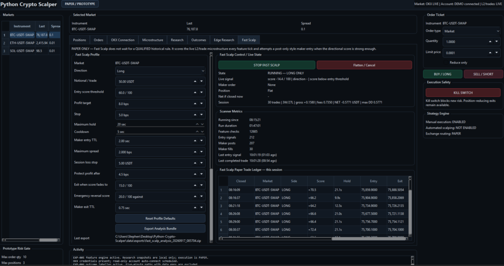
Market data
Level 2
Trade tape
Feature values
Positions
Orders
Trading configuration
Strategy state
Paper trades
Scanner metrics
Market viability

Supporting smaller laptop screens was unexpectedly painful.

Desktop layouts that looked perfectly good on a large monitor became almost unusable on a 14 or 15-inch laptop.

The application now has a more aggressive compact mode that hides secondary panels such as the manual order ticket and activity log when space is limited.

I also had to explicitly disable mouse-wheel changes on trading controls.

Accidentally changing a stop loss because the mouse happened to be hovering over a numeric field while scrolling is not exactly ideal behaviour for a trading application.

Where the project goes next

The next stage is not simply “turn on real trading.”

There is still a lot to prove.

The current focus is establishing whether there is a repeatable edge after execution costs.

Some of the questions we are investigating now include:

Does the activity gate significantly improve MFE?
Which volatility regimes produce the best trades?
Are maker fills suffering from adverse selection?
Is Long-only structurally stronger for this signal?
What is the optimum hold duration?
Is the current score weighting correct?
Should the strategy dynamically change its target based on current volatility?
Can a maker-first exit model materially reduce fee drag?
How closely will simulated fills match real exchange behaviour?

Only after the paper strategy demonstrates credible positive expectancy would moving to automated demo exchange orders make sense.

And only after that behaves correctly would real capital even become a discussion.

The biggest lesson so far

When people think about algorithmic trading, they tend to focus on finding the perfect indicator.

That has not been the hardest part of this project.

The much harder problem is:

Finding a movement large and reliable enough that something remains after fees, spread, slippage and imperfect execution.

A model can correctly predict that Bitcoin is about to move up.

That prediction is worthless if Bitcoin moves 0.01% and trading the move costs 0.05%.

That distinction has changed the direction of the project significantly.

Instead of asking:

“Can we predict the next tiny price movement?”

the better question is becoming:

“Can we identify the moments where both direction and sufficient opportunity exist?”

That is a considerably more interesting problem.

And that is where the project currently stands.